Seeing Superposition

May 23, 2026 · finished · likely

I’ve been doing mech-interp for some time and “superposition” kept appearing in everything I read. I had a basic sense of the term and wrote a brief explanation post. Still, the best way to comprehend something is to see the thing with your own eyes. So I decided to replicate the experiment from Elhage et al., 2022 (notebook). It’s not the whole paper, but specifically $W^T W$ heatmap. I wanted to see superposition emerge from training and address a few questions I had while replicating the experiment — specifically why non-linearity matters and what off-diagonal patterns are actually showing.

Before we even try to visualize and see superposition in practice, we need to identify what kind of data we should be working with. We have the following premises regarding data that’ll lead to interpretable results:

Sparsity: most features we observe in practice rarely occur.
Features > Model dimensions: a constraining factor that forces the model to compress.
Feature Importance: not all features are equally important for a given task.

We set up a small model with $n = 20$ and $m = 5$ , where $n$ is the number of features and $m$ is the number of dimensions our model has. We also need to vary the sparsity level and assign different importance to each feature.

As for the synthetic data, the input vectors $x$ simulate the mentioned premises. Every $x_i$ (which is a “feature”) has an associated sparsity $S$ and importance $I_i$ . Every $x_i$ equals $0$ with probability $S$ and is uniformly distributed between $[0, 1]$ otherwise. As for the importance, the paper uses geometric decay: $I_i = 0.7^i$ . $0.7$ is an arbitrarily chosen base and isn’t a magic number. Looking at $I$ :

I = \begin{bmatrix} 1.0 & 0.7 & 0.49 & 0.34 & 0.24 & \dots & 0.7^{19} \end{bmatrix}

Importance affects the loss — errors on more significant features are penalized more heavily, so the model prioritizes representing them. The loss is:

\mathcal{L} = \sum_{i=0}^{n-1} I_i (x_i - \hat{x}_i)^2

Now that we have identified the loss function — what exactly are we trying to minimize the loss for?

The model tries to reconstruct the embeddings of $x$ with $n$ features via $m$ -dimensional space. The model looks like this:

\begin{aligned} h &= W x \\ \hat{x} &= \operatorname{ReLU}(W^T h + b) \\ &= \operatorname{ReLU}(W^T W x + b) \end{aligned}

The paper hypothesis suggests that every feature in the $n$ -dimensional space can be represented in the lower $m$ -dimensional one. We are using linear map $W$ , where $W \in \mathbb{R}^{m \times n}$ is the weight matrix. Each column $W_i$ represents the direction of the feature $x_i$ .

We use the transpose of the matrix $W^T$ to recover the original vector.

We also include bias to the recovered result. The reason for doing so is to allow the model to nudge the features to their expected values.

Analytical insight

Besides showing the actual loss $\mathcal{L}$ that would be computed while training, the paper analytically explains why superposition is occuring showing this equation:

\mathbb{E}_x[\mathcal{L}] \sim \underbrace{\sum_i I_i \left(1 - \|W_i\|^2\right)^2}_{\text{feature benefit}} + \underbrace{\sum_{i \neq j} I_j \left(W_j \cdot W_i\right)^2}_{interference}

Feature benefit is the value a model gains from representing a feature.

Interference is the noise value between $x_i$ and $x_j$ embeddings that are non-orthogonal to each other.

Full deriviation: from MSE to feature benefit + interference

We start deriving from our original MSE loss:

\mathcal{L} = \sum_{i=0}^{n-1} I_i (x_i - \hat{x}_i)^2

Now we start substituting the value of $\hat{x}_i$ relative to the $x$ :

\hat{x}_i = (W^T W x)_i

Knowing that $(W^T W)_{ij} = W_i \cdot W_j$ we replace matrix multiplication with explicit sum:

\begin{aligned} \hat{x}_i &= (W^T W x)_i \\ &= \sum_{j} (W^T W)_{ij} x_j \\ &= \sum_{j} (W_i \cdot W_j) x_j \\ &= (W_i \cdot W_i) x_i + \sum_{i \neq j} (W_i \cdot W_j) x_j \\ \end{aligned}

Since $W_i \cdot W_i = \lVert W_i \rVert^2$ we substitute that for $i = j$ case:

\begin{aligned} \hat{x}_i &= \lVert W_i \rVert^2 x_i + \sum_{i \neq j} (W_i \cdot W_j) x_j \end{aligned}

Following the original loss equation:

\begin{aligned} x_i - \hat{x}_i &= x_i - \lVert W_i \rVert^2 x_i - \sum_{i \neq j} (W_i \cdot W_j) x_j \\ &= x_i (1 - \lVert W_i \rVert^2) - \sum_{i \neq j} (W_i \cdot W_j) x_j \\ \mathcal{L} &= \sum_{i} I_i \left( x_i (1 - \lVert W_i \rVert^2) - \sum_{j \neq i} (W_i \cdot W_j) x_j \right)^2 \\ &= \sum_{i} I_i \Bigg[ \underbrace{x_i^2 (1 - \lVert W_i \rVert^2)^2}_{\text{(A)}} \;-\; \underbrace{2 x_i (1 - \lVert W_i \rVert^2) \sum_{j \neq i} (W_i \cdot W_j) x_j}_{\text{(B)}} \;+\; \underbrace{\Bigg(\sum_{j \neq i} (W_i \cdot W_j) x_j\Bigg)^2}_{\text{(C)}} \Bigg] \end{aligned}

Now we take the expectation $\mathbb{E}_x[\mathcal{L}]$ . The standard assumption in the toy model is that features are independent with $\mathbb{E}[x_i] = 0$ and $\mathbb{E}[x_i x_j] = 0$ for $i \neq j$ , while $\mathbb{E}[x_i^2]$ is some constant (typically normalized so it acts as $1$ , which is why it disappears below — if you don’t normalize, just carry it through as a scalar).

Term (A) survives directly:

\mathbb{E}[x_i^2 (1 - \lVert W_i \rVert^2)^2] = (1 - \lVert W_i \rVert^2)^2

Term (B) vanishes, because every summand contains $\mathbb{E}[x_i x_j]$ with $i \neq j$ , which is zero:

\mathbb{E}\!\left[2 x_i (1 - \lVert W_i \rVert^2) \sum_{j \neq i} (W_i \cdot W_j) x_j\right] = 0

Term (C) simplifies because the cross terms $\mathbb{E}[x_j x_k] = 0$ for $j \neq k$ , leaving only the diagonal:

\mathbb{E}\!\left[\Bigg(\sum_{j \neq i} (W_i \cdot W_j) x_j\Bigg)^{\!2}\right] = \sum_{j \neq i} (W_i \cdot W_j)^2

Putting (A), (B), and (C) back together:

\mathbb{E}_x[\mathcal{L}] = \sum_{i} I_i (1 - \lVert W_i \rVert^2)^2 + \sum_{i} I_i \sum_{j \neq i} (W_i \cdot W_j)^2

The second double sum is over pairs $(i, j)$ with $i \neq j$ , which we can rewrite as $\sum_{i \neq j}$ . The paper indexes the importance on the interfering feature $j$ rather than $i$ (a relabeling — both forms appear in the literature), giving the form quoted at the top:

\mathbb{E}_x[\mathcal{L}] \sim \underbrace{\sum_i I_i (1 - \lVert W_i \rVert^2)^2}_{\text{feature benefit}} + \underbrace{\sum_{i \neq j} I_j (W_i \cdot W_j)^2}_{\text{interference}}

The $\sim$ rather than $=$ absorbs the $\mathbb{E}[x_i^2]$ constant from the normalization assumption.

Visualization

W^T W across different sparsities

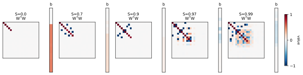
Across the panels we’re looking at $W^T W$ which is the matrix of pairwise dot products between feature directions.

As sparsity increases, it starts to represent more features — but more interference also emerges. The diagonal $\lVert W_i \rVert^2$ is influencing the feature benefit cost while off-diagonals $W_i \cdot W_j$ are affecting the interference cost.

We see that in the densest case ( $S = 0$ ), only diagonal entries are highlighted for the 5 most important features. As sparsity increases, more diagonal entries light up. At the same time more off-diagonals show up. By $S = 0.97$ and $S = 0.99$ , we see that a dense block forms in the bottom-right — the low-importance features group together while the high-importance features maintain cleaner directions.

The model forms these patterns because as sparsity rises, interference is paid less in the expectation (because features fire less often when sparse), so the model can represent more features at the cost of letting them share directions.

The thing that is worth noting is the colors of the off-diagonals. The colors aren’t arbitrary — red means $W_i \cdot W_j > 0$ (pointing in similar directions), blue means $W_i \cdot W_j < 0$ (pointing in opposite directions).

We see that in the earlier heatmaps the off-diagonal cells are strongly blue. They form because the model arranges these feature directions as antipodal pairs — two feature directions pointing in exactly opposite directions, so $W_i \cdot W_j = -1$ .

This actually answers a question I had been sitting with: why does the model need a non-linearity to superpose? Here’s why. When feature $j$ fires and contaminates feature $i$ ‘s readout, an antipodal arrangement makes that contamination negative. ReLU clips it to zero, thus clearing the interference for free. Without ReLU, antipodal pairs would buy the model nothing — squared dot product is the same in either direction.

As the sparsity rises, we see red cells emerge. This is when angles between directions become acute and the model accepts non-cleanable interference because the features causing it are low-importance and rarely fire. The model can’t keep using antipodal arrangement since it can only have a limited number of them. For example, if we try to fit 5 features into 2 dimensions, geometry forces some pairs into acute angles.

Conclusion

Before the replication I’d say that I had a little understanding of how the model tries to compress $n$ features into $m < n$ hidden dimensions. Now I’d say it’s about using non-linearity to filter cheap interference; superposition is the consequence.

The paper covers a lot more than this one experiment. I’m especially curious about geometric organization of features in superposition and how phase transitions occur between configurations.